A Neat Error Function Approximation
In this post, we’re going to try to approximate the error function, which is a very important function in statistics and also a fascinating function overall. I wanted to make this post for a long time now because it combines ideas from mathematics and computer science, and it even introduces a new idea as well! If you are ready, let’s dive in.
If you don’t remember, the error function is defined as below. $$erf(x) = \frac{2}{\sqrt{\pi}} \int_{0}^{x} e^{-t^{2}} dt $$
Unfortunately, the antiderivative of \(e^{-t^{2}}\) cannot be expressed in terms of elementary functions, hence why we have the error function in the first place.
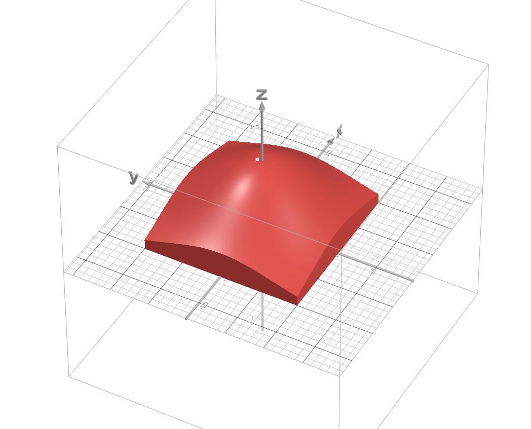
But the integral we are going to focus on is a bit different, precisely; $$I(t)=\int_{-t}^{t}e^{-x^{2}}dx$$ which is equal to \(\sqrt{\pi} erf(t)\). If you don’t know how to find the whole area under the curve \(e^{-x^{2}}\), the next step might be ambiguous. So I recommend checking the classic method of finding the said area first. If you are ready, let’s look at \(I^{2}(t)\) $$I^{2}(t)=\int_{-t}^{t}e^{-x^{2}}dx \int_{-t}^{t}e^{-x^{2}}dx=\int_{-t}^{t}e^{-x^{2}}dx \int_{-t}^{t}e^{-y^{2}}dy=\int_{-t}^{t}\int_{-t}^{t}e^{-(x^{2}+y^{2})}dydx$$ Here’s the graph of this function. Unfortunately, I couldn’t get Geogebra to render a 3D volume, so I’ll put an image below. But you can play around with the 3D graph using this desmos link.

If you pay attention to the region we are integrating over, it is a square with the side length of \(2t\). And since it is a square, we can’t utilize the polar coordinates to find a precise formula for the area. But what we can do is, we can draw two circular regions, one that is inscribed by our square region and one that inscribes our square region to set bounds for our integral. Their radius are \(t\) and \(t\sqrt{2}\) respectively. (Keep in mind that the below inequality holds for \(t \geq 0\), but this is not a big issue because the \(erf(t)\) is an odd function. Meaning for \(t \lt 0\), we can just use \(-erf(-t)\))
$$\int_{-t}^{t}\int_{-\sqrt{t^{2}-x^{2}}}^{\sqrt{t^{2}-x^{2}}}e^{-(x^{2}+y^{2})}dydx \leq I^{2}(t) \leq \int_{-t\sqrt{2}}^{t\sqrt{2}}\int_{-\sqrt{2t^{2}-x^{2}}}^{\sqrt{2t^{2}-x^{2}}}e^{-(x^{2}+y^{2})}dydx$$
The integrals may look scary, but since their region is circular, we can use polar coordinates to simplify and even solve them. We are going to let \(x=r \cos(\theta)\) and \(y=r \sin(\theta)\). And the Jacobian determinant is; $$ \begin{vmatrix} J \end{vmatrix} = \begin{vmatrix} \frac{\partial{x}}{\partial{r}} & \frac{\partial{x}}{\partial{\theta}} \\ \frac{\partial{y}}{\partial{r}} & \frac{\partial{y}}{\partial{\theta}} \end{vmatrix} = \cos{\theta} \cdot r\cos{\theta} - (-r\sin{\theta}) \cdot \sin{\theta} = r (\sin^{2}{\theta} + \cos^{2}{\theta})=r$$
Thus, our inequality becomes
$$\int_{0}^{2\pi}\int_{0}^{t} e^{-r^{2}} r dr d\theta \leq I^{2}(t) \leq \int_{0}^{2\pi}\int_{0}^{t\sqrt{2}} e^{-r^{2}} r dr d\theta$$
To evaluate the integrals we are going to apply a single u-substitution, precisely \(u=r^2\). The rest is pretty trivial, so I’ll leave it as an exercise to you and just write down the result.
$$ \pi (1 - e^{-t^{2}}) \leq I^{2}(t) \leq \pi (1 - e^{-2t^{2}}) $$ $$ \sqrt{\pi} \cdot \sqrt{1 - e^{-t^{2}}} \leq I(t) \leq \sqrt{\pi} \cdot \sqrt{1 - e^{-2t^{2}}} $$
And recall that \(I(t) = \sqrt{\pi} erf(t)\)
$$ \sqrt{1-e^{-t^{2}}} \leq erf(t) \leq \sqrt{1-e^{-2t^{2}}} $$
Attempt #1: Simple Linear Regression
We are going to try to approximate the error function as a linear combination of the terms \(\sqrt{1-e^{-x^2}}\), \(\sqrt{1-e^{-2x^2}}\) and \(1\). $$ erf(x) \approx w_{1}\sqrt{1-e^{-x^2}} + w_{2}\sqrt{1-e^{-2x^2}} + b $$
Before trying to find \(w_{1}\) and \(w_{2}\), we can put some constraints on them. Our first constraint will arise after taking a limit as \(x \to \infty\) $$ \lim_{x \to \infty}{erf(x)} = \lim_{x \to \infty}{w_{1}\sqrt{1-e^{-t^2}} + w_{2}\sqrt{1-e^{-2t^2}}} + b $$ $$ 1 = w_{1} + w_{2} + b $$
To get our second constraint we’ll just substitute \(x = 0\) $$ erf(0) \approx w_{1}\sqrt{1-e^{-0^2}} + w_{2}\sqrt{1-e^{-2 \cdot 0^2}} + b $$ $$ 0 = b $$
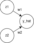
Now, for the regression, I am going to use a neural network with 2 neurons in its input layers with bias disabled, 1 neuron in its output layer and no hidden layers. For the training set, I’ll generate random \(x\) values between \(0\) and \(2\), (PS: I used the range \(\left[0, 1\right]\) in all of my attempts, but later on found that using the range \(\left[0, 2\right]\) gives more accurate approximations), apply functions \(\sqrt{1-e^{-x^2}}\) and \(\sqrt{1-e^{-2x^2}}\) to those \(x\) values and feed that to the neural network. So, it will think that there is a linear connection between input and output when in reality there isn’t. I am also going to use mean squared error as my loss function and stochastic gradient descent as my optimizer. Surprisingly SGD optimizer performs better than Adam optimizer for this task.
If you don’t know anything about neural networks, they essentially process their inputs by passing them through layers of the network, which involves matrix multiplications and activation function applications. After this, they calculate a loss value to quantify the error between the predicted output and the actual target. Based on this loss value, they adjust the elements of the matrices (weights) using optimization algorithms, which are responsible for updating the weights to minimize the loss
Here, \(y\) is a vector of true values and \(\hat{y}\) is a vector of prediction values. So with everything said, our network is ready, it is pretty simple but effective.

I used TensorFlow Keras to train it, here’s the code.
def fun(x, exponent):
    return np.sqrt(1 - np.exp(-exponent * x * x))

class SumToOneConstraint(tf.keras.constraints.Constraint):
    def __init__(self):
        pass

    def __call__(self, w):
        return w / tf.reduce_sum(w)

exponent_1 = 1
exponent_2 = 2

N = 10000
x_train = np.random.uniform(0, 2, (N, 1))
y_train = erf(x_train)
x_train = np.column_stack((
    fun(x_train, exponent_1),
    fun(x_train, exponent_2)
))

initial_learning_rate = 0.1
scheduler = ReduceLROnPlateau(monitor='loss', factor=0.1, patience=3, min_lr=1e-7)

# Build model
i = Input(shape=(2,))
x = Dense(1, use_bias=False, kernel_constraint=SumToOneConstraint())(i)

model = Model(i, x)
model.compile(
    # optimizer=Adam(learning_rate=initial_learning_rate),
    optimizer=SGD(learning_rate=initial_learning_rate, momentum=0.0),
    loss='mse',
)

# Train the model and print results
r = model.fit(x_train, y_train, epochs=20, callbacks=[scheduler])
weights = model.get_weights()[0].flatten()

print(f"Weight 1: {weights[0]}, Exponent 1: {exponent_1}")
print(f"Weight 2: {weights[1]}, Exponent 2: {exponent_2}")
And after running it for a couple of epochs it produces okay-ish results.

But I didn’t stop there.
Attempt #2: “Better” Exponents
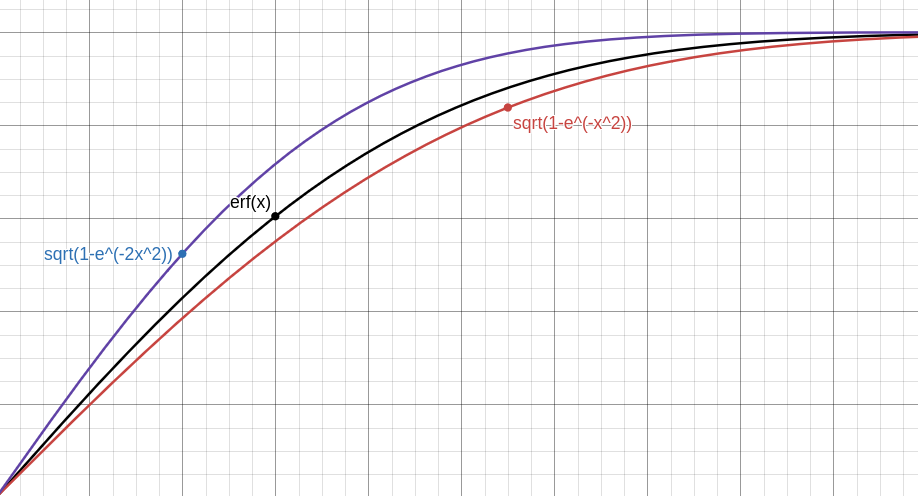
If you check graph of \(\sqrt{1-e^{-x^2}}\), \(\sqrt{1-e^{-2x^2}}\) and \(erf(x)\) you’ll see that functions are not that close

We can definitely find closer functions, one that satisfies the inequality \(\sqrt{1-e^{-a_{1}x^2}} \lesssim erf(x)\) and the other that satisfies \(erf(x) \lesssim \sqrt{1-e^{-a_{2}x^2}}\) for some \(a_{1}\) and \(a_{2}\). To find \(a_{1}\) and \(a_{2}\), I’ll use good old binary search.
The algorithm is simple, we’re going to pick the middle point on a predefined range \(\left[low, high\right]\), and we’ll alter the bounds of that range
based on whether the midpoint satisfies the necessary condition or not. I’ll also be using the mpmath library to avoid floating point precision errors.
from mpmath import mpf, mp
import mpmath

mp.dps = 50

delta = mpf("1e-5")
x_beg = mpf("0")
x_end = mpf("2.5")

def fun(x, a):
    return mpmath.sqrt(1 - mpmath.exp(-a * x * x))

def find_lower_bound(low, high, iterations):
    mid = 0
    for i in range(iterations):
        mid = (low + high) / 2
        print(f"Iteration: {i + 1}, exponent: {mid}")
        x = x_beg
        while x <= x_end:
            if fun(x, mid) > mpmath.erf(x):
                high = mid
                break
            x += delta
        else:
            low = mid
    return mid

print(find_lower_bound(1, 1.5, 55))
from mpmath import mpf, mp
import mpmath

mp.dps = 50

delta = mpf("1e-5")
x_beg = mpf("0")
x_end = mpf("2.5")

def fun(x, a):
    return mpmath.sqrt(1 - mpmath.exp(-a * x * x))

def find_upper_bound(low, high, iterations):
    mid = 0
    for i in range(iterations):
        mid = (low + high) / 2
        print(f"Iteration: {i + 1}, exponent: {mid}")
        x = x_beg
        while x <= x_end:
            if fun(x, mid) < mpmath.erf(x):
                low = mid
                break
            x += delta
        else:
            high = mid
    return mid

print(find_upper_bound(1, 1.5, 55))
After running those programs we find \(a_{1}=1.138219454220815\) and \(a_{2}=1.2732395447313372\). So let’s use these as our exponents and train. We should get better results, right?

Welp, that didn’t help.
Attempt #3: Testing Random Exponents And Picking The Ones With The Lowest Error
The last attempt was a big failure, but it did give us a new perspective. Turns out the functions don’t have to be numerically close to \(erf(x)\) to approximate it better. To find better exponents what I am going to do is, I’ll generate random exponent pairs along with random \(x\) values and use those to produce my training data. Then, after training my model, I’ll manually calculate the error value of each exponent pair, sort the exponents list by their error values and take, say, first 100 values. That was a bit mouthful but not much changes in terms of code.
# ...
N = 30000
exponents_1 = np.random.uniform(1, 1.138219454220815, (N, 1))
exponents_2 = np.random.uniform(1.2732395447313372, 2, (N, 1))

x_train = np.random.uniform(0, 2, (N, 1))
y_train = erf(x_train)
x_train = np.column_stack((
    fun(x_train, exponents_1),
    fun(x_train, exponents_2)
))
# ...
# Train the model
r = model.fit(x_train, y_train, epochs=10, callbacks=[scheduler])
weights = model.get_weights()[0].flatten()
w0, w1 = weights

# Find best exponents
exponents = np.column_stack((exponents_1, exponents_2))

correct_values = y_train
errors = []
for e1, e2 in exponents:
    y_hat = w0 * fun(x_train, e1) + w1 * fun(x_train, e2)
    mse = np.linalg.norm(y_hat - correct_values) / N
    errors.append([mse, e1, e2])

errors = np.array(errors)
indices = np.argsort(errors[:, 0])
sorted_errors = errors[indices][:100]

print(f"Mean 1: {sorted_errors[:, 1].mean()}")
print(f"STD 1: {sorted_errors[:, 1].std()}")

print(f"Mean 2: {sorted_errors[:, 2].mean()}")
print(f"STD 2: {sorted_errors[:, 2].std()}")
Let’s train the model. Below you’ll see the mean and standard deviation of the first \(100\) best exponent values.

You can ignore the loss values, since we used random exponents and most of them are not great. But we did get some interesting results. Surprisingly the second exponent value is very close to \(2\). Let’s train the model with these as the exponents.

That’s an improvement, but I had one last thing up my sleeve.
Attempt #4: Learning The Exponents
The last step was a big improvement, but it wasn’t that interesting when I was initially testing my models on \(\left[0, 1\right]\). So I had to further improve my approximation. So far I’ve trained my model to learn the values \(w_{1}\) and \(w_{2}\). What if I could make it learn \(a_{1}\) and \(a_{2}\) as well? For a loss function \(L\), all I needed was a way to calculate \(\frac{\partial{L}}{\partial{a_{1}}}\) and \(\frac{\partial{L}}{\partial{a_{2}}}\), the rest is gradient descent.
Let’s focus on \(\frac{\partial{L}}{\partial{a_{1}}}\) first. We can use chain rule to work our way back one step, below \(\hat{y_{i}}\) represents our prediction.
$$ \frac{\partial{L}}{\partial{\hat{a_{1}}}} = \frac{\partial{L}}{\partial{\hat{y_{i}}}}\frac{\partial{\hat{y_{i}}}}{\partial{a_{1}}} $$
The first term on right-hand side is computable, we used the mean squared error which has the formula $$L(\hat{y})=MSE(\hat{y})=\frac{1}{N}\sum_{i=1}^{N}\left(y_{i} - \hat{y_{i}}\right)^{2} $$
So that means $$\frac{\partial{L}}{\partial{\hat{y_{i}}}} = \frac{-2}{N} \sum_{i=1}^{N} \left(y_{i}-\hat{y_{i}}\right) $$
PS: If the subscript \(i\) confuses you, please remember that \(\hat{y}\) is not a single prediction but a vector of predictions since when training a model we use fixed batches of data. So the \(\hat{y_{i}}\) there represents the current prediction.
And we know that we can write our prediction as $$\hat{y_{i}} = w_{1}z_{1} + w_{2}z_{2}$$
for $$ z_{1} = \sqrt{1-e^{-a_{1}x^2}} \text{ and } z_{2} = \sqrt{1-e^{-a_{2}x^2}} $$
So we can apply the chain rule one last time to find the value of \(\frac{\partial{\hat{y_{i}}}}{\partial{a_{1}}}\) $$ \frac{\partial{\hat{y_{i}}}}{\partial{a_{1}}} = \frac{\partial{\hat{y_{i}}}}{\partial{z_{1}}}\frac{\partial{z_{1}}}{\partial{a_{1}}} = w_{1}\frac{\partial{z_{1}}}{\partial{a_{1}}} $$ $$ \frac{\partial{z_{1}}}{\partial{a_{1}}} = \frac{x^2 e^{-a_{1}x^2}}{2\sqrt{1-e^{-a_{1}x^2}}} $$
We can take similar steps to show that we can backpropagate our loss to \(a_{2}\), but it is pretty trivial, so I won’t show it here. But this result means we can actually learn the exponents!
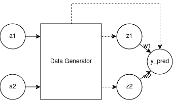
By knowing that, I’ve created a new artificial neural network architecture that I’ve never seen before. I’m not saying that I am the first person that have used something like this, but the closest thing I could find was something called hypernetworks. I really wanted to call it “Network in Network” but unfortunately that exact name is already taken, so I am open for suggestions.
But anyway, let’s focus on our new network. It is not complex either, we’re going to have a data generator network followed by our old network. To learn the exponents, we’re going to generate the data, train the old network, propagate final loss back to the data generator network and repeat.

I couldn’t get our exponents to be learned automatically using keras API (skill issue), so we are going to do it manually. Also, by experimentation, I found out that by keeping inner epochs to a minimum, we tend to learn better, but be careful because if you set the inner epochs too low you might be a subject to exploding gradients problem. I have also modified the initial exponent values by hand because these new values produce better approximation. Down below, you can check the code the results.
def fun(x, exponent):
    return np.sqrt(1 - np.exp(-exponent * x * x))

def fun_derivative(x, exponent):
    return x * x * np.exp(-exponent * x * x) / (2 * fun(x, exponent))

class SumToOneConstraint(tf.keras.constraints.Constraint):
    def __init__(self):
        pass

    def __call__(self, w):
        return w / tf.reduce_sum(w)


def generate_data(e0, e1, N):
    xs = np.random.uniform(0, 2, (N, 1))
    Y = erf(xs)
    X = np.column_stack((
        fun(xs, e0),
        fun(xs, e1)
    ))

    return xs, X, Y

e0 = 1.137
e1 = 1.86

N = 10_000  # Row count of the train dataset
inner_network_epochs = 4
outer_network_epochs = 20
initial_inner_learning_rate = 0.10
outer_learning_rate = 0.05
w0, w1 = 0, 0

lr_decay_rate = 0.00

i = Input(shape=(2,))
x = Dense(1, use_bias=False, kernel_constraint=SumToOneConstraint())(i)
model = Model(i, x)

for outer_epoch in range(outer_network_epochs):
    print(f"Ou)
    if outer_epoch > outer_network_epochs - 5:
        inner_network_epochs = 20
    inner_learning_rate = initial_inner_learning_rate

    xs, X, Y = generate_data(e0, e1, N)
    model.compile(
        # optimizer=Adam(learning_rate=inner_learning_rate),
        optimizer=SGD(learning_rate=inner_learning_rate, momentum=0.0),
        loss='mse'
    )

    r = model.fit(X, Y, epochs=inner_network_epochs)
    weights = model.get_weights()[0].flatten()
    w0, w1 = weights

    y_hat = w0 * X[:, 0] + w1 * X[:, 1]
    mse_derivative = 2 * np.mean(Y.flatten() - y_hat)

    grad_e0 = np.sum((mse_derivative * w0 * fun_derivative(xs, e0)).flatten())
    grad_e1 = np.sum((mse_derivative * w1 * fun_derivative(xs, e1)).flatten())

    # SGD
    e0 = e0 - outer_learning_rate * grad_e0
    e1 = e1 - outer_learning_rate * grad_e1

    print(f"Exponents: {e0}, {e1}")
    print(f"Weights: {w0}, {w1}")

Marvelous! Let’s calculate the max absolute error.
from mpmath import mpf, mp
import mpmath

mp.dps = 50

delta = mpf("1e-5")
x_beg = mpf("0")
x_end = mpf("4")

e0 = 1.1037659365451735
e1 = 1.855694042069345
w0 = 0.7507712841033936
w1 = 0.24922874569892883

def fun(x, a):
    return mpmath.sqrt(1 - mpmath.exp(-a * x * x))

def approx(x):
    return w0 * fun(x, e0) + w1 * fun(x, e1)

x = x_beg
max_error = mpf("0")
x_error = mpf("0")

while x < x_end:
    error = mpmath.erf(x) - approx(x)
    if error < 0:
        error = -error

    if error > max_error:
        max_error = error
        x_error = x
    x += delta

print(f"Exponents: {e0} {e1}")
print(f"Weights: {w0} {w1}")
print(f"Max error: {max_error}")
print(f"At x={x_error}")

So the absolute error is about \(5\cdot10^{-5}\) which is pretty nice, it beats an approximation that is on the Wikipedia page for the error function and comes really close to another one. I’ve had a lot of fun working on this and writing this blog post. Here’s a desmos link if you want to play with the formula yourself.